Quick introduction to AI

Since this is the very first article in this blog, I thought it would be good to give some really basic info what this blog is about and what neural networks are. This article also contains the very first shitty algorithm I implemented using a neural network. Let’s get started!

There are tons of neural network tutorials out there already, I’m not really going into depth with this. If you want something more hands on, I would recommend checking out the Google’s machine learning crash course

What is a neural network?

Neural network, or more specifically artificial neural network (ANN) is a mathematical formula designed to “learn” how to get from a given input to an output. The input and output values both must be numerals, but there are ways to turn, for example, an image to a matrix of numbers.

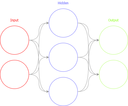
ANN contains of multiple neurons and connections between them. Each node and a connection have a value set to them called a “weight”. When the network is activated, each neuron “vote” about which of its connections should be activated.

A very basic code example

Since I’m usually using Tensorflow, most of the code examples in this blog will be using it. You can install prebuilt Tensorflow with Python pip: pip install tensorflow, or if you have NVidia GPU with Cuda cores and Cuda supported drivers, pip install tensorflow-gpu

Let’s create a neural network algorithm, that predicts how a bitwise XOR would work. If you don’t remember what it does, it takes 2 binary inputs and outputs a single bit according to the following table:

Training dataset

Usually training data contains for thousands or hundreds of thousands of examples, but since we’re doing such a simple implementation, 4 examples should be enough.

1
2
3
4
5
6
7
8
9
10
11

import tensorflow as tf

training_data = [
    (0, 0, 0),
    (1, 0, 1),
    (0, 1, 1),
    (1, 1, 0)
]

x = [(i[0], i[1]) for i in training_data]
y = [i[2] for i in training_data]

Now x contains tuple of inputs and y contains outputs.

Creating a basic model

1
2
3
4
5
6

model = tf.keras.models.Sequential([
    tf.keras.layers.Dense(8, input_dim=2, activation='relu'),
    tf.keras.layers.Dense(1, activation='sigmoid'),
])
model.compile(tf.keras.optimizers.Adam(learning_rate=0.001),
                loss='mean_squared_error')

Here we are using Tensorflow’s Keras-api, which is what I use for my projects. It allows you to stack layers easily and keep the code simple. We are using a model with 2 inputs: input_dim=2, which has 1 hidden layer with 8 neurons. Each neuron is connected to the input and output automatically. The activation function we’re using is relu, which is a simple mathematical formula to filter the input. If the input is less than 0, the output is zero and if the input is more than zero, the output is the same as input. This is used to improve the learning rate of the neural network.

The last layer is the output and there we are using the sigmoid-function, which is used to smooth out the output. Since the output is just a single neuron, we can directly read the output and round it to closest whole number, 0 or 1.

The last thing to do is compile the model to something we can use. Here we’re using the Adam-optimizer. Since I’m not an expert of this, you can read more about the Adam algorithm here. Optimizer’s task is to train the network so it will find the proper weights for the neurons. Imagine standing in the middle of a field, blindfolded, and your task is to find the lowest point of the field. You can do this by taking small steps in random direction and trying to figure out if it’s lower than from were you started. The learning_rate -parameter is the size of these steps and loss is simply put what you are trying to achieve, for example, trying to find the lowest spot.

Training the network

Now that our model and training data is all set up, we can train the model. This is done with the fit-method of the model:

1

model.fit(x=x, y=y, epochs=300)

Here the x-parameter is the input and y is the output we’re trying to achieve. epochs is number of training steps done to train the model. After some testing, 300 seemed to work for this example. There is always a correct answer for the number of training steps, but you’ll never know it without trying.

Let’s add some validation at the end of the code to see if it works.

1
2

print(['{} XOR {} = {}'.format(
    x[0], x[1], model.predict([x])[0][0].round()) for x in x])

Running the code

1
2
3
4
5
6
7
8
9
10
11
12
13
14
15
16
17
18
19
20
21
22
23
24
25
26
27
28
29
30
31

$ python xor.py
2020-03-04 01:37:39.054976: I tensorflow/stream_executor/platform/default/dso_loader.cc:44] Successfully opened dynamic library cudart64_101.dll
2020-03-04 01:37:41.291890: I tensorflow/stream_executor/platform/default/dso_loader.cc:44] Successfully opened dynamic library nvcuda.dll

# ...snip...

Train on 4 samples
Epoch 1/300

4/4 [==============================] - 0s 117ms/sample - loss: 0.2867
Epoch 2/300

4/4 [==============================] - 0s 1ms/sample - loss: 0.2863
Epoch 3/300

4/4 [==============================] - 0s 1ms/sample - loss: 0.2859
Epoch 4/300

4/4 [==============================] - 0s 1ms/sample - loss: 0.2855
Epoch 5/300

# ...snip...

4/4 [==============================] - 0s 1ms/sample - loss: 0.2026
Epoch 299/300

4/4 [==============================] - 0s 1ms/sample - loss: 0.2023
Epoch 300/300

4/4 [==============================] - 0s 1ms/sample - loss: 0.2020
['0 XOR 0 = 1.0', '1 XOR 0 = 1.0', '0 XOR 1 = 1.0', '1 XOR 1 = 0.0']

You can see the loss drop over time. This means we’re getting closer to the wanted prediction. The smaller the loss is, the better the network does its thing.

But wait, 0 XOR 0 definately should not be 1! Oh well, this is what the blog is all about. You can find the whole code example from here and you can run it with python xor.py

So will it AI? Yes, probably, if you give it enough training!